|
|
 |
9. Transition and Turbulence
This section was adapted from The Engine and the Atmosphere: An
Introduction to Engineering by Z. Warhaft, Cambridge University Press, 1997.
9.1 Laminar flow and transition
How many times a day do we turn on a faucet? Do it now. First very slowly,
and you will see glassy, orderly flow. If there is no wind or other disturbance,
nothing will change. This is called laminar flow. A photo taken now will be
identical to one taken half an hour later. Such a flow is deterministic;
information about its future behavior is completely determined by specification
of the flow at an earlier time. Now open the faucet to full on, or better still
open a fire hydrant, or watch a smoke stack. Here, for this faster or larger
scale motion, the flow pattern is changing all the time. Although its average
motion is in one direction (sideways for the fire-hydrant, up for the smoke
stack), within the flow there are irregularities everywhere. For example if you
could train your eyes on a small speck of dust it would certainly move along but
it would jitter as well, sometimes darting to one side, or up or down. Turbulent
flow while proceeding in a particular direction, like laminar flow, has the
added complexity of random velocity fluctuations. The flow patterns never repeat
themselves. To convince yourself of this watch a smoke stack for a few minutes.
Fluid flow that is slow tends to be laminar. As it speeds up a transition
occurs and it crinkles up into complicated, random turbulent flow. But even
slow flow coming from a large orifice can be turbulent; this is the case with
smoke stacks. Engineers and scientists don't like to say "fast" or "slow"
or "small" and "big" since there is no reference. Small compared to what?
Big compared to what? Since turbulence is altogether a different type of
fluid flow to laminar flow, it is desirable to be able to quantify under what
conditions it occurs.
 |
|
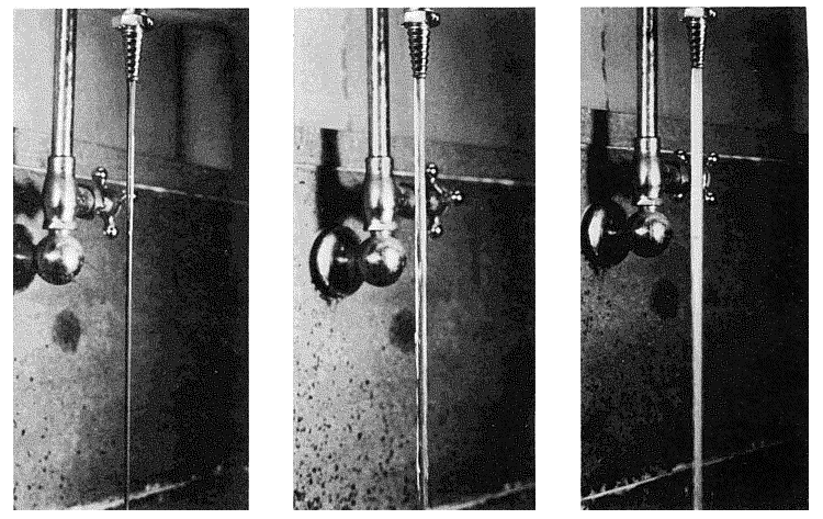
Figure 9.1 Laminar, transitional, and turbulent flow from a faucet.
From Engineering Fluid Mechanics, A. Mironer, MacGraw-Hill, 1979.
|
Let us re-do the faucet experiment in a more systematic way. We have shown
that as the speed, V, increases, transition to turbulence will occur.
Now, instead of using water in your pipes, replace it with honey. Assuming
you could provide a large enough pressure, even for fast flow the motion
would remain laminar. If you do not wish to do this experiment, stir a
spoon rapidly in a cup of water and then at the same speed (working hard)
in a cup of honey. Honey has a higher viscosity than water and the viscosity
resists transition to turbulence: while the water is turbulent, the honey remains
laminar at the same speed. Finally, put a nozzle on your tap and constrict
the water flow into a fine glass capillary tube. Here too the flow can be made
to go quite fast without it becoming turbulent. Our experiments suggest
that laminar flow occurs for low speeds, small diameters, low densities and high
viscosities, while turbulent flows occur for the opposite conditions: high speeds, large
diameters, high densities and low viscosities. Now viscosity is a measurable fluid property
(as is its density, temperature, etc.). We will discuss it more in a moment, but we often
use the "kinematic viscosity," which is the viscosity divided by the density. Its unit is
m^2/s. Notice its dimensions are the same as a length multiplied by a velocity. If the
fluid speed is V (m/s), the orifice diameter is d (m) then we can write the
following dimensionless ratio
Re is the Reynolds number, named after Osborne Reynolds who
did systematic experiments, of a similar type to those described above, one
hundred years ago. Notice that if V or d (or both) are small and the viscosity is
large, Re will be small. For this case the flow will be laminar. Increase d
or V or decrease the viscosity, and Re will increase. Reynolds found that for flow
in a pipe it did not matter which of the three particular parameters he varied
in this dimensionless group: as long as Re was less than approximately 2300,
the flow was laminar. Above this value, turbulence would invariably occur.
This is a general result since it allows us to vary the type of fluid, flow
speed and pipe diameter without having to use the words "large" or "fast,"
etc. Moreover, since Re is dimensionless, it does not matter which system
of units are used (S.I., Engineering, etc.) so long as they are the same
throughout. We can now talk of high Reynolds number flow or low Reynolds number
pipe flow, knowing that in this context low means somewhat less than 2000. The
kinematic viscosity of water is approximately 10^{-6} m^2/s (that of honey is about
10^{-3} m^2/s, 1000 times greater than that of water). Thus if the pipe
diameter is say 1 cm, the speed at which the Reynolds number is 2000, is 0.2 m/s or approximately 0.4 mph, a rather
slow speed. Water undergoes
transition to turbulence at low speeds. Most of the water flows we see,
such as in streams and rivers, are indeed turbulent.
Air too is a fluid, its viscosity, \nu, is approximately 10^{-3} m^2/s.
This is a higher viscosity than that of water. This rather counter-intuitive fact is
due to the great differences in density of the two fluids. Water has a density
of approximately 1000 kg/m^3; the air density is 1.2 \, kg/m^3. Thus
part of the "viscous feeling" we have when we pull our fingers through
water is really due to inertia --- we are having to move the water away from our
hands and this also provides resistance. For this reason we need to remember the
difference between the dynamic viscosity and the kinematic viscosity.
The dynamic viscosity of water is approximately
10^{-3} kg/(m s) while that of air is 1.2 \times 10^{-5} kg/(m s). Thus the
dynamic viscosity of water is higher than that of air, in keeping with our
intuitive notion.
 While the transition from laminar to turbulent flow occurs at a Reynolds
number of approximately 2300 in a pipe, the precise value depends on whether
any small disturbances are present. If the experiment is very carefully
arranged so that the pipe is very smooth and there are no disturbances to the
velocity and so on, higher values of Re can be obtained with the flow still in
a laminar state. However, if Re is less than 2300, the flow will be laminar
even if it is disturbed. Thus 2300 is the value the Re below which turbulence
will not occur in a pipe. Moreover, if the flow has a different geometry, such
as flow in a square duct, or over a turbine blade, transition will occur at
different values of Re. The essential point is that flows become turbulent at
high Reynolds numbers where "high" means much greater than unity.
While the transition from laminar to turbulent flow occurs at a Reynolds
number of approximately 2300 in a pipe, the precise value depends on whether
any small disturbances are present. If the experiment is very carefully
arranged so that the pipe is very smooth and there are no disturbances to the
velocity and so on, higher values of Re can be obtained with the flow still in
a laminar state. However, if Re is less than 2300, the flow will be laminar
even if it is disturbed. Thus 2300 is the value the Re below which turbulence
will not occur in a pipe. Moreover, if the flow has a different geometry, such
as flow in a square duct, or over a turbine blade, transition will occur at
different values of Re. The essential point is that flows become turbulent at
high Reynolds numbers where "high" means much greater than unity.
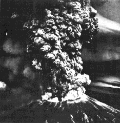
Air motion is invariably turbulent. Consider a smokestack (which to a
first approximation is mostly air). If its diameter is say 3 m, then V
must be less than 6.6 mm/s (0.015 mph) for it to be laminar! There is
no such thing as a laminar smokestack. Clouds too are usually turbulent. Here we
determine the Reynolds number using an approximate characteristic dimension of
the cloud such as its height or width. Assuming the cloud dimension is say 500 m, and its
characteristic internal motion is say 5 m/s, then taking the kinematic viscosity to be 10^{-5} m^2/s
(it is approximately the same for water vapor as it is for air), the
Re = (500 x 5)/10^{-5} = 2.5 x 10^8. A high value indeed. No wonder
cumulus clouds always have a random, puffy looking turbulent
structure (see also the plume generated by Mt. St. Helens in the picture above).
9.2 Turbulent Flow
When the flow is
turbulent, the flow contains eddying motions of all sizes, and a large part of the
mechanical energy in the flow goes into the formation of these eddies which eventually
dissipate their energy as heat. As a result, at a given Reynolds number, the drag of a
turbulent flow is higher than the drag of a laminar flow. Also, turbulent flow is
affected by surface roughness, so that increasing roughness increases the drag.
Transition to turbulence can occur over a range of Reynolds numbers, depending on many
factors, including the level surface roughness, heat transfer, vibration, noise, and
other disturbances. To understand why this is so, and to appreciate the role of the
Reynolds number in governing the stability of the flow, it is helpful to think in terms
of a spring-damper system such as the suspension system of a car. Driving along a bumpy
road, the springs act to reduce the movement experienced by the passengers. If there
were no shock absorbers, however, there would be no damping of the motion, and the car
would continue to oscillate long after the bump has been left behind. So the shock
absorbers, through a viscous damping action, dissipate the energy in the oscillations and
reduce the amplitude of the oscillations. If the viscous action is strong enough, the
oscillations will die out very quickly, and the passengers can proceed smoothly. If
the shock absorbers are not in good shape, the oscillations may not die out. The
oscillations can actually grow if the excitation frequency is in the right range, and the
system can experience resonance. The car becomes unstable, and it is then virtually
uncontrollable.
In fluid flow, we often interpret the Reynolds number as the ratio of the inertia force
(that is, the force given by mass x acceleration) to the viscous force. At low Reynolds numbers, therefore, the viscous
force is large compared to the inertia force, and the flow behaves in some ways like a
car with a good suspension system. Small disturbances in the velocity field, created
perhaps by small roughness elements on the surface, or pressure perturbations from
external sources such as vibrations in the surface or strong sound waves, will be
damped out and not allowed to grow. This is the case for pipe flow at
Reynolds numbers less than the critical value of 2300 (based on pipe diamter and average velocity),
and for boundary layers with a Reynolds number less than about 200,000 (based on distance from the
origin of the layer and the freestream velocity). As the Reynolds number
increases, however, the viscous damping action becomes comparatively less, and at some
point it becomes possible for small perturbations to grow, just as in the case of a car
with poor shock absorbers. The flow can become unstable, and it can experience
transition to a turbulent state where large variations in the velocity field can be
maintained. If the disturbances are very small, as in the case where the surface is very
smooth, or if the wavelength of the disturbance is not near the point of resonance, the
transition to turbulence will occur at a higher Reynolds number than the critical
value. So the point of transition does not correspond to a single Reynolds number, and
it is possible to delay transition to relatively large values by controlling the
disturbance environment. At very high Reynolds numbers, however, it is not
possible to maintain laminar flow since under these conditions even minute disturbances will
be amplified into turbulence.
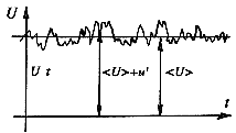
Turbulent flow is characterized by unsteady eddying motions that are in constant motion
with respect to each other. At any point in the flow, the eddies produce fluctuations
in the flow velocity and pressure. If we were to measure the streamwise velocity
in turbulent pipe flow, we would see a variation in time as shown in
figure 9.2.
 |
|
Figure 9.2 Velocity at a point in a turbulent flow as a function of time.
|
We see that the velocity has a time-averaged value \bar U
and a fluctuating value u', so that \bar U is not a function of
time, but u' is.
The eddies interact with each other as they move around, and they can exchange momentum
and energy. For example, an eddy that is near the centerline of the pipe (and therefore
has a relatively high velocity), may move towards the wall and interact with eddies near
the wall (which typically have lower velocities). As they mix, momentum differences are
smoothed out. This process is superficially similar to the action of viscosity which
tends to smooth out momentum gradients by molecular interactions, and turbulent flows are
sometimes said to have an equivalent eddy viscosity. Because turbulent mixing is
such an effective transport process, the eddy viscosity is typically several
orders of magnitude larger than the molecular viscosity. The important point is that
turbulent flows are very effective at mixing: the eddying motions can very quickly
transport momentum, energy and heat from one place to another. As a result, velocity
differences get smoothed out more effectively than in a laminar flow, and the
time-averaged velocity profile in a turbulent flow is much more uniform than in
a laminar flow (see figure 11.1).
As a result of this mixing, the velocity gradient at the wall is higher than that seen
in a laminar flow at the same Reynolds number, so that the shear stress at the wall is
correspondingly larger. This observation is in agreement with the fact that the losses
in a turbulent flow are much higher than in a laminar flow, and therefore the pressure
drop per unit length will be greater, which is reflected in a larger frictional stress
at the wall.
|
|